Arranjo Fatorial de Tratamentos
Programa SAS
data fatorial;
input Genero $ Categ $ IMC;
cards;
F AT 19.7
F AT 20.3
F AT 19.3
F AT 20.9
F SEM 22.4
F SEM 21.9
F SEM 23.8
F SEM 24.1
F SED 26.3
F SED 23.5
F SED 24.8
F SED 26.6
F PR 26.2
F PR 24.2
F PR 25.4
F PR 24.9
M AT 20.2
M AT 21.3
M AT 19.3
M AT 21.1
M SEM 21.2
M SEM 20.1
M SEM 19.7
M SEM 21.1
M SED 27.3
M SED 23.4
M SED 25.2
M SED 26.4
M PR 22.3
M PR 22.2
M PR 22.1
M PR 23.3
;
proc print;
run;
Proc glm;
class Genero Categ;
model IMC = Genero Categ Genero*Categ;
lsmeans Genero*Categ / slice=Genero adjust=tukey PDIFF=all;
lsmeans Genero*Categ / slice=Categ adjust=tukey PDIFF=all;
run;
Variações do programa:
Proc glm;
class Genero Categ;
model IMC = Genero Categ Genero*Categ;
lsmeans Genero*Categ / slice=Genero adjust=tukey PDIFF=all;
lsmeans Genero*Categ / slice=Categ adjust=tukey PDIFF=all;
/*
lsmeans Categ;
means Categ / Tukey lines;
means Genero*Categ / tukey lines;
*/
run;
Para Calculo de Efeitos Principais:
Proc anova;
class Genero Categ;
model IMC = Genero Categ Genero*Categ;
means Categ / Tukey lines;
run;
Arquivo de Saida (Tipo Word) para download:


Fazer os gráficos no Excel utilizando tabela dinâmica.


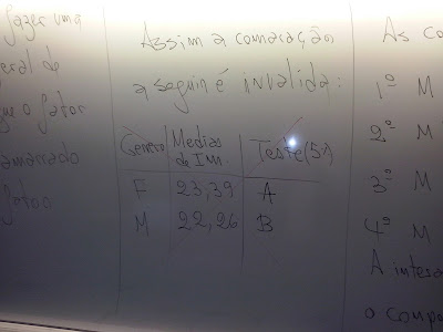
Podemos ver que os gráficos são diferentes, e que as concussões estatísticas também o são.
Veja que no gráfico do gênero feminino professor e sedentário não diferem (as duas barras, medias aritméticas tem a letra A).
No gratifico do Gênero Masculino as categorias Sedentário Professor diferem (Sedentário tem letra A e Professor letra B).


Foto das Louças Onde Discutimos os Resultados


Exemplo Sem Interação Significativa
Autora: Ana Carolina Donofre (Dados simulados)
data fatorial;
input Linhagem $ Densidade $ GP;
cards;
C 10 2.44
C 10 2.39
C 10 2.42
C 10 2.45
C 14 2.03
C 14 1.99
C 14 2.05
C 14 2.07
C 18 1.78
C 18 1.83
C 18 1.81
C 18 1.73
R 10 2.37
R 10 2.30
R 10 2.34
R 10 2.38
R 14 1.88
R 14 1.90
R 14 1.87
R 14 1.92
R 18 1.65
R 18 1.69
R 18 1.70
R 18 1.67
;
proc print;
run;
Proc glm;
class Linhagem Densidade;
model GP = Linhagem Densidade Linhagem*Densidade;
lsmeans Linhagem*Densidade / slice=Linhagem adjust=tukey PDIFF=all;
lsmeans Linhagem*Densidade/ slice=Densidade adjust=tukey PDIFF=all;
means Linhagem / Tukey lines;
means Densidade / Tukey lines;
run;
Arquivo para Download Sem Interação:
Resultados SAS Sem Interação
Outro Exemplo Sem Interação
Outro Exemplo Sem Interação
data consumo;
input Trat $ Imp $ Cons;
cards;
1 a 17.2
1 a 18.3
1 a 17.5
1 a 18.4
1 b 20.3
1 b 21.3
1 b 22.1
1 b 19.5
2 a 22.1
2 a 23.5
2 a 24.5
2 a 21.5
2 b 25.5
2 b 26.4
2 b 27.3
2 b 26.1
3 a 20.2
3 a 23.2
3 a 21.5
3 a 20.1
3 b 22.2
3 b 22.3
3 b 24.5
3 b 26.1
4 a 19.8
4 a 18.8
4 a 19.5
4 a 20.2
4 b 24.3
4 b 23.4
4 b 22.1
4 b 22.7
;
proc print;
run;
proc glm;
class Trat Imp;
model Cons = Trat Imp Trat*Imp;
lsmeans Trat*Imp / slice=Trat adjust=tukey PDIFF=all;
lsmeans Trat*Imp / slice=Imp adjust=tukey PDIFF=all;
run;
/*
means Trat / tukey lines;
means Imp / tukey lines;
*/
Saida:
| The SAS System |
| Obs | Trat | Imp | Cons |
|---|---|---|---|
| 1 | 1 | a | 17.2 |
| 2 | 1 | a | 18.3 |
| 3 | 1 | a | 17.5 |
| 4 | 1 | a | 18.4 |
| 5 | 1 | b | 20.3 |
| 6 | 1 | b | 21.3 |
| 7 | 1 | b | 22.1 |
| 8 | 1 | b | 19.5 |
| 9 | 2 | a | 22.1 |
| 10 | 2 | a | 23.5 |
| 11 | 2 | a | 24.5 |
| 12 | 2 | a | 21.5 |
| 13 | 2 | b | 25.5 |
| 14 | 2 | b | 26.4 |
| 15 | 2 | b | 27.3 |
| 16 | 2 | b | 26.1 |
| 17 | 3 | a | 20.2 |
| 18 | 3 | a | 23.2 |
| 19 | 3 | a | 21.5 |
| 20 | 3 | a | 20.1 |
| 21 | 3 | b | 22.2 |
| 22 | 3 | b | 22.3 |
| 23 | 3 | b | 24.5 |
| 24 | 3 | b | 26.1 |
| 25 | 4 | a | 19.8 |
| 26 | 4 | a | 18.8 |
| 27 | 4 | a | 19.5 |
| 28 | 4 | a | 20.2 |
| 29 | 4 | b | 24.3 |
| 30 | 4 | b | 23.4 |
| 31 | 4 | b | 22.1 |
| 32 | 4 | b | 22.7 |
| The SAS System |
The ANOVA Procedure
| Class Level Information | ||
|---|---|---|
| Class | Levels | Values |
| Trat | 4 | 1 2 3 4 |
| Imp | 2 | a b |
| Number of Observations Read | 32 |
|---|---|
| Number of Observations Used | 32 |
| The SAS System |
The ANOVA Procedure
Dependent Variable: Cons
| Source | DF | Sum of Squares | Mean Square | F Value | Pr > F |
|---|---|---|---|---|---|
| Model | 7 | 196.0700000 | 28.0100000 | 20.53 | <.0001 |
| Error | 24 | 32.7500000 | 1.3645833 | ||
| Corrected Total | 31 | 228.8200000 |
| R-Square | Coeff Var | Root MSE | Cons Mean |
|---|---|---|---|
| 0.856874 | 5.321885 | 1.168154 | 21.95000 |
| Source | DF | Anova SS | Mean Square | F Value | Pr > F |
|---|---|---|---|---|---|
| Trat | 3 | 117.2475000 | 39.0825000 | 28.64 | <.0001 |
| Imp | 1 | 77.5012500 | 77.5012500 | 56.79 | <.0001 |
| Trat*Imp | 3 | 1.3212500 | 0.4404167 | 0.32 | 0.8088 |
| The SAS System |
The ANOVA Procedure
| The SAS System |
The ANOVA Procedure
Tukey's Studentized Range (HSD) Test for Cons
| Note: | This test controls the Type I experimentwise error rate, but it generally has a higher Type II error rate than REGWQ. |
| Alpha | 0.05 |
|---|---|
| Error Degrees of Freedom | 24 |
| Error Mean Square | 1.364583 |
| Critical Value of Studentized Range | 3.90126 |
| Minimum Significant Difference | 1.6112 |
| Means with the same
letter are not significantly different. | |||
|---|---|---|---|
| Tukey Grouping | Mean | N | Trat |
| A | 24.6125 | 8 | 2 |
| B | 22.5125 | 8 | 3 |
| B | |||
| B | 21.3500 | 8 | 4 |
| C | 19.3250 | 8 | 1 |
| The SAS System |
The ANOVA Procedure
| The SAS System |
The ANOVA Procedure
Tukey's Studentized Range (HSD) Test for Cons
| Note: | This test controls the Type I experimentwise error rate, but it generally has a higher Type II error rate than REGWQ. |
| Alpha | 0.05 |
|---|---|
| Error Degrees of Freedom | 24 |
| Error Mean Square | 1.364583 |
| Critical Value of Studentized Range | 2.91879 |
| Minimum Significant Difference | 0.8524 |
| Means with the same
letter are not significantly different. | |||
|---|---|---|---|
| Tukey Grouping | Mean | N | Imp |
| A | 23.5063 | 16 | b |
| B | 20.3938 | 16 | a |
| The SAS System |
| Obs | Trat | Imp | Cons |
|---|---|---|---|
| 1 | 1 | a | 17.2 |
| 2 | 1 | a | 18.3 |
| 3 | 1 | a | 17.5 |
| 4 | 1 | a | 18.4 |
| 5 | 1 | b | 20.3 |
| 6 | 1 | b | 21.3 |
| 7 | 1 | b | 22.1 |
| 8 | 1 | b | 19.5 |
| 9 | 2 | a | 22.1 |
| 10 | 2 | a | 23.5 |
| 11 | 2 | a | 24.5 |
| 12 | 2 | a | 21.5 |
| 13 | 2 | b | 25.5 |
| 14 | 2 | b | 26.4 |
| 15 | 2 | b | 27.3 |
| 16 | 2 | b | 26.1 |
| 17 | 3 | a | 20.2 |
| 18 | 3 | a | 23.2 |
| 19 | 3 | a | 21.5 |
| 20 | 3 | a | 20.1 |
| 21 | 3 | b | 22.2 |
| 22 | 3 | b | 22.3 |
| 23 | 3 | b | 24.5 |
| 24 | 3 | b | 26.1 |
| 25 | 4 | a | 19.8 |
| 26 | 4 | a | 18.8 |
| 27 | 4 | a | 19.5 |
| 28 | 4 | a | 20.2 |
| 29 | 4 | b | 24.3 |
| 30 | 4 | b | 23.4 |
| 31 | 4 | b | 22.1 |
| 32 | 4 | b | 22.7 |
| The SAS System |
The GLM Procedure
| Class Level Information | ||
|---|---|---|
| Class | Levels | Values |
| Trat | 4 | 1 2 3 4 |
| Imp | 2 | a b |
| Number of Observations Read | 32 |
|---|---|
| Number of Observations Used | 32 |
| The SAS System |
The GLM Procedure
Dependent Variable: Cons
| Source | DF | Sum of Squares | Mean Square | F Value | Pr > F |
|---|---|---|---|---|---|
| Model | 7 | 196.0700000 | 28.0100000 | 20.53 | <.0001 |
| Error | 24 | 32.7500000 | 1.3645833 | ||
| Corrected Total | 31 | 228.8200000 |
| R-Square | Coeff Var | Root MSE | Cons Mean |
|---|---|---|---|
| 0.856874 | 5.321885 | 1.168154 | 21.95000 |
| Source | DF | Type I SS | Mean Square | F Value | Pr > F |
|---|---|---|---|---|---|
| Trat | 3 | 117.2475000 | 39.0825000 | 28.64 | <.0001 |
| Imp | 1 | 77.5012500 | 77.5012500 | 56.79 | <.0001 |
| Trat*Imp | 3 | 1.3212500 | 0.4404167 | 0.32 | 0.8088 |
| Source | DF | Type III SS | Mean Square | F Value | Pr > F |
|---|---|---|---|---|---|
| Trat | 3 | 117.2475000 | 39.0825000 | 28.64 | <.0001 |
| Imp | 1 | 77.5012500 | 77.5012500 | 56.79 | <.0001 |
| Trat*Imp | 3 | 1.3212500 | 0.4404167 | 0.32 | 0.8088 |
| The SAS System |
The GLM Procedure
Least Squares Means
Adjustment for Multiple Comparisons: Tukey
| Trat | Imp | Cons LSMEAN | LSMEAN Number |
|---|---|---|---|
| 1 | a | 17.8500000 | 1 |
| 1 | b | 20.8000000 | 2 |
| 2 | a | 22.9000000 | 3 |
| 2 | b | 26.3250000 | 4 |
| 3 | a | 21.2500000 | 5 |
| 3 | b | 23.7750000 | 6 |
| 4 | a | 19.5750000 | 7 |
| 4 | b | 23.1250000 | 8 |
| Least Squares Means for effect
Trat*Imp Pr > |t| for H0: LSMean(i)=LSMean(j) Dependent Variable: Cons | ||||||||
|---|---|---|---|---|---|---|---|---|
| i/j | 1 | 2 | 3 | 4 | 5 | 6 | 7 | 8 |
| 1 | 0.0282 | <.0001 | <.0001 | 0.0080 | <.0001 | 0.4493 | <.0001 | |
| 2 | 0.0282 | 0.2256 | <.0001 | 0.9992 | 0.0263 | 0.8087 | 0.1378 | |
| 3 | <.0001 | 0.2256 | 0.0074 | 0.5036 | 0.9593 | 0.0099 | 1.0000 | |
| 4 | <.0001 | <.0001 | 0.0074 | <.0001 | 0.0803 | <.0001 | 0.0141 | |
| 5 | 0.0080 | 0.9992 | 0.5036 | <.0001 | 0.0855 | 0.4853 | 0.3489 | |
| 6 | <.0001 | 0.0263 | 0.9593 | 0.0803 | 0.0855 | 0.0008 | 0.9923 | |
| 7 | 0.4493 | 0.8087 | 0.0099 | <.0001 | 0.4853 | 0.0008 | 0.0052 | |
| 8 | <.0001 | 0.1378 | 1.0000 | 0.0141 | 0.3489 | 0.9923 | 0.0052 | |
| The SAS System |
The GLM Procedure
Least Squares Means
| Trat*Imp Effect Sliced by Trat for Cons | |||||
|---|---|---|---|---|---|
| Trat | DF | Sum of Squares | Mean Square | F Value | Pr > F |
| 1 | 1 | 17.405000 | 17.405000 | 12.75 | 0.0015 |
| 2 | 1 | 23.461250 | 23.461250 | 17.19 | 0.0004 |
| 3 | 1 | 12.751250 | 12.751250 | 9.34 | 0.0054 |
| 4 | 1 | 25.205000 | 25.205000 | 18.47 | 0.0002 |
| The SAS System |
The GLM Procedure
Least Squares Means
Adjustment for Multiple Comparisons: Tukey
| Trat | Imp | Cons LSMEAN | LSMEAN Number |
|---|---|---|---|
| 1 | a | 17.8500000 | 1 |
| 1 | b | 20.8000000 | 2 |
| 2 | a | 22.9000000 | 3 |
| 2 | b | 26.3250000 | 4 |
| 3 | a | 21.2500000 | 5 |
| 3 | b | 23.7750000 | 6 |
| 4 | a | 19.5750000 | 7 |
| 4 | b | 23.1250000 | 8 |
| Least Squares Means for effect
Trat*Imp Pr > |t| for H0: LSMean(i)=LSMean(j) Dependent Variable: Cons | ||||||||
|---|---|---|---|---|---|---|---|---|
| i/j | 1 | 2 | 3 | 4 | 5 | 6 | 7 | 8 |
| 1 | 0.0282 | <.0001 | <.0001 | 0.0080 | <.0001 | 0.4493 | <.0001 | |
| 2 | 0.0282 | 0.2256 | <.0001 | 0.9992 | 0.0263 | 0.8087 | 0.1378 | |
| 3 | <.0001 | 0.2256 | 0.0074 | 0.5036 | 0.9593 | 0.0099 | 1.0000 | |
| 4 | <.0001 | <.0001 | 0.0074 | <.0001 | 0.0803 | <.0001 | 0.0141 | |
| 5 | 0.0080 | 0.9992 | 0.5036 | <.0001 | 0.0855 | 0.4853 | 0.3489 | |
| 6 | <.0001 | 0.0263 | 0.9593 | 0.0803 | 0.0855 | 0.0008 | 0.9923 | |
| 7 | 0.4493 | 0.8087 | 0.0099 | <.0001 | 0.4853 | 0.0008 | 0.0052 | |
| 8 | <.0001 | 0.1378 | 1.0000 | 0.0141 | 0.3489 | 0.9923 | 0.0052 | |
| The SAS System |
The GLM Procedure
Least Squares Means
| Trat*Imp Effect Sliced by Imp for Cons | |||||
|---|---|---|---|---|---|
| Imp | DF | Sum of Squares | Mean Square | F Value | Pr > F |
| a | 3 | 56.621875 | 18.873958 | 13.83 | <.0001 |
| b | 3 | 61.946875 | 20.648958 | 15.13 | <.0001 |
Nenhum comentário:
Postar um comentário